Sensitivity analysis

Just finished taking a really useful ICPSR summer workshop on sensitivity analysis with Kenneth Frank. Thought I'd share a few learnings.
Dr. Frank's team has built an app for calculating the robustness of inference to replacement statistic (RIR; for continuous and dichotomous outcomes) and the impact threshold for a confounding variable (ITCV; for continuous outcomes) that can be accessed online at https://konfound-project.shinyapps.io/konfound-it/. There is also a package version for R and Stata called konfound.
# r code
install.packages("konfound")

* stata code
ssc install konfound
The RIR "quantifies what proportion of the data must be replaced (with cases with zero effect) to make the estimated effect have a p-value of .05."
The ITCV "reports how strongly an omitted variable would have to be correlated with both the predictor of interest and the outcome to make the estimated effect have a p-value of .05."
For a metric similar to ITCV but for dichotomous outcomes, a calculator for VanderWeele's e-value (expressed in risk ratio format) is available online at https://www.evalue-calculator.com/evalue/ or through the EValue package for R and the evalue package for Stata.
# r code
install.packages("EValue")

* stata code
ssc install evalue
The e-value is "defined as the minimum strength of association on the risk ratio scale that an unmeasured confounder would need to have with both the exposure and the outcome, conditional on the measured covariates, to fully explain away a specific exposure-outcome association."
Here is a quick worked example using youth risk behavior survey data looking at the association between gun carrying and suicide attempt outcomes in a paper we published here.
From our model, we get the estimate in log odds 1.881, the standard error .154, the sample size 38,619, and the number of covariates (20).
To get the RIR, we need one additional number, which is the number of cases in the treatment condition (2,530):
. tab gun

                  gun |      Freq.     Percent        Cum.
----------------------+-----------------------------------
Did not carry firearm |     48,863       95.08       95.08
      Carried firearm |      2,530        4.92      100.00
----------------------+-----------------------------------
                Total |     51,393      100.00
We can then compute the RIR using the pkonfound function and receive this helpful interpretive output:
. pkonfound 1.881362 .1541601 38619 20 2530, model_type(1)

Robustness of Inference to Replacement (RIR):

RIR = 47

The table implied by the parameter estimates and sample sizes you entered:

             |      Fail    Success  Success_%
-------------+--------------------------------
     Control |     35951        138    .382388
   Treatment |      2468         62   2.450593
       Total |     38419        200   .5178798

The reported effect size = 1.881362, SE = .1541601, p-value = 0.000
Values have been rounded to the nearest integer. This may cause small change to the
estimated effect for the table.

To invalidate the inference that the effect is different from 0 (alpha = .05) one would
need to replace 47 (75.806%) treatment success data points with data points for which
the probability of failure in the entire sample (93.091%) applies (RIR = 47). This is
equivalent to transferring 46 data points from treatment success to treatment failure
(Fragility = 46).

Note that RIR = Fragility/[1-P(success in the entire sample)

The transfer of 46 data points yields the following table:

             |      Fail    Success  Success_%
-------------+--------------------------------
     Control |     35951        138    .382388
   Treatment |      2514         16   .6324111
       Total |     38465        154   .3987674

Effect size = 0.506, SE = 0.265, p-value = 0.056
This is based on t = estimated effect/standard error
Note, in this case the data is weighted, thus we make an additional assumption that each replaced case would have an average sampling weight (or any other combination of sampling weights, as long as they add up to 47).
We might write up the results as something like:
To help quantify the robustness of the inference, the robustness of inference to replacement metric was calculated (RIR; Frank, 2000). To invalidate the inference, 75.8% of positive cases would need to be replaced from the sample population. Assuming each replacement case had an average sampling weight, 47 datapoints in the treatment group would need to be replaced from the sample population. This is equivalent to a fragility index of 46.
To then calculate the e-value, we'll need the model estimate in odds ratio form (6.562) with the 95% confidence intervals of the estimate [4.841, 8.896]: We can then calculate the e-value of our estimate and get a nice figure of the result:
. evalue or 6.562437, lcl(4.84106) ucl(8.895899) figure
   E-value (point estimate): 12.604
   E-value (CI): 9.153
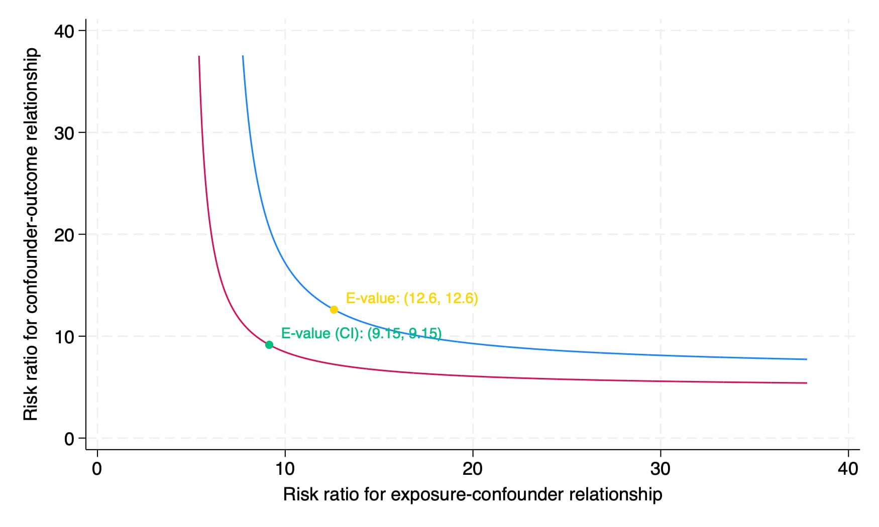
Here, 12.6 is the e-value for the point estimate and 9.15 is the more conservative e-value for the lower confidence limit. Although we do not get as much helpful interpretive output as we do in the pkonfound command, using the help evalue documentation, we can adapt their suggested language to the following:
To help quantify the robustness of the estimate, the e-value was calculated (VanderWeele & Ding, 2017). An unmeasured confounder associated with suicide attempts and gun-carrying by a risk ratio of 9.15-fold each could explain away the lower confidence limit, but weaker confounding could not.
So there you have it! Both app websites (and the related package documentation) have a lot of further resources and references on these techniques. There are probably subtitles I am missing here and I am certainly no expert, but I think these tools are relatively easy to implement and could really help strengthen an understanding of how robust a result is. Also, you by no means need the actual data to calculate these statistics – these same steps could easily be used to estimate the robustness of an inference/estimate from published studies.
Postscript: At the time of writing, the Stata konfound package available via ssc install is not the most updated version and the command used in this post will not run with the current ssc version until the updates are released. However, all the same information can be entered into https://konfound-project.shinyapps.io/konfound-it/ or run with the R package command pkonfound(1.881, 0.154, 38619, 20, n_treat = 2530, model_type = 'logistic') to get the same results.
